Model Training and Evaluation

This lab provides an introduction to training, modifying, and evaluating machine learning models for radar perception, using a Generalizable Radar Transformer (GRT) reference implementation. In this lab, you will:

1. Get access to GPUs via an HPC system, and run cluster jobs
2. Set up a model training environment
3. Replicate the GRT baselines, and measure how performance scales with the size of the training set
4. Propose and implement a change to the model or the training methodology
5. Run an ablation to evaluate your change against the baselines

Report Template

Please use this template for your lab report.

Revision History

Date	Description
2026-09-06	Initial draft
2026-09-12	Added the evaluation section, report template, and rubric
2026-09-15	Officially released and assigned

Hello World, HPC!

None of the models in this lab (and, most likely, in your course project) can be trained on a laptop. Instead, they require access to accelerators such as GPUs, ideally in a high-performance computing (HPC) environment.

In this checkpoint (Due 09/22), you should verify that you are able to log into PSC, use our allocation, and submit a hello_world.sh slurm job.

Bring Your Own Compute

You are welcome (and encouraged) to use your own (≥16GB VRAM) GPU instead of the PSC allocation, provided you also have at least 2TB of free storage. If you elect to do so, you may skip this checkpoint. Instead, submit the following:

1. A screenshot of your compute environment and accelerators (e.g., nvidia-smi, scontrol show nodes, etc.).

2. Download the I/Q-1M dataset using these instructions, and submit a screenshot showing that you have downloaded the dataset to your computing environment.

   Note that you only need the radar and lidar range files; you can --exclude */lidar/rfl */lidar/nir */_camera/video.avi so that the dataset only consumes ~2TB of storage.

On the flip side, if you are planning to use your own compute, you are also welcome (and encouraged) to follow these PSC setup steps regardless in case you need to fall back to the PSC allocation.

• Your GPU should have at least 16GB of VRAM, though it is possible to use GPUs with less memory with aggressive memory management (e.g., gradient accumulation); note that we will not help you do this.
• V100s will be very slow, but usable.
• You may also use TPUs, Trainium, Apple Silicon, etc.; however, software support may vary, and we will not provide technical support.

Provided that you have created an NSF Access account and submitted your username to the canvas assignment, you should have been added to the course allocation ele260011p on PSC Bridges-2:

Log in to PSC

Follow the instructions in the PSC Bridges-2 user guide to log in to the cluster.

• I highly recommend registering your public key; see the instructions under "Public-private keys".
• Once you log in, you should see our course allocation displayed (similar to the screenshot above); you can also pull this up at any time using the projects command.

VS Code Remote Editor on PSC

PSC supports running VS Code directly on a compute node, which is far more pleasant than editing over ssh. This is not required, but we strongly recommend setting it up now, before you need it; see the remote IDE instructions in the user guide.

Submit a job

Following the sbatch instructions in the PSC user guide, create a "hello world" script which runs the following commands:

echo "Hello World, HPC!"
echo
echo "job id:    ${SLURM_JOB_ID}"
echo "partition: ${SLURM_JOB_PARTITION}"
echo "account:   ${SLURM_JOB_ACCOUNT}"
echo "node:      $(hostname)"
echo "user:      $(whoami)"
echo "date:      $(date)"

Your script should also do the following:

• Set a reasonable job name (e.g., hello_world).
• Use the RM-small partition, and be billed to our course allocation ele260011p.
• Save the output to a log file (e.g., hello_world.%j.log)

Once you create your script, run it with

sbatch hello_world.sh

Sample Output

You should get an output that looks something like this:

[tianshu2@bridges2-login013 ~]$ cat hello_world.45378265.log
Hello World, HPC!

job id:    45378265
partition: RM-small
account:   ele260011p
node:      r001.ib.bridges2.psc.edu
user:      tianshu2
date:      Sun Sep  6 17:04:25 EDT 2026

Note that if the script is not routed through slurm via sbatch, you will instead see:

[tianshu2@bridges2-login013 ~]$ ./helloworld.sh
Hello World, HPC!

job id:
partition:
account:
node:      br013.ib.bridges2.psc.edu
user:      tianshu2
date:      Sun Sep  6 17:07:29 EDT 2026

Once you are done, submit a screenshot of the projects output and the log file from your hello_world.sh job to the Lab 2 Checkpoint assignment on canvas.

Set up the Training Environment

Using your compute environment, you should now set up the training environment for this lab. Unless noted otherwise, these steps are the same whether you are on PSC or on your own machine.

1. Install uv. uv is a modern python version and package manager which is open source, extremely fast, built to a high quality standard, and, for better or worse, now fully owned by OpenAI as a loss leader.

   curl -LsSf https://astral.sh/uv/install.sh | sh
   

2. Clone the repository, and make it your own. Create a new, empty, private repository under your personal GitHub account, then point your clone at it and push:

   git clone https://github.com/RadarML/18848-lab2.git --recursive
   cd 18848-lab2
   git remote set-url origin git@github.com:<your-username>/18848-lab2.git
   git push -u origin main
   

   Warning

   Make sure that your repository is private!

3. Install the dependencies. Run uv sync in the repository root.

   Warning

   This downloads several GB of packages, and can be painfully slow on a login node. If it is, run it from an interactive session instead:

   interact -A ele260011p --ntasks-per-node=16
   

4. Install the pre-commit hooks. This will run a number of checks on your code before each commit, helping catch errors early.

   uv run pre-commit install
   

5. Link the dataset. The repository looks for the dataset at ./data by default.

   • On PSC, point that at the shared copy (i.e., create a symlink):

     ln -s /ocean/projects/ele250004p/shared/data/iq1m/ data
     

     Info

     Note that the dataset lives under ele250004p, which is not our course allocation. This is intended — the data is shared from another project, and you only need read access to it.

   • On your own machine, point it to wherever you downloaded the dataset. See above, as well as the i/q-1m documentation for instructions on downloading the dataset.

   It is also possible to simply pass meta.dataset=/full/path/to/dataset each time you run train.py and --data_root=/full/path/to/dataset each time you run evaluate.py, but it's much more convenient to use a symlink.

Verify your Installation

Start an interactive session (i.e., interact -A ele260011p --ntasks-per-node=16), and run a "dry-run" of the training script from the interactive session:

uv run train.py meta.name=debug meta.version=v0 meta.dry_run=inst

• When you run train.py with meta.dry_run=inst, this will instantiate all of the components without actually loading any data or running any training, allowing you to easily verify that all dependencies are installed and importable, and that there are no immediate errors during instantiation.
• This process does load metadata though, providing a useful sanity check of the entire data pipeline configuration.

Sample Output

[tianshu2@r002 18848-lab2]$ uv run train.py meta.name=debug meta.version=v0 meta.dry_run=inst
Using bfloat16 Automatic Mixed Precision (AMP)
GPU available: False, used: False
TPU available: False, using: 0 TPU cores
HPU available: False, using: 0 HPUs
[09/06/26 17:35:33] INFO     train: Dry run (inst): instantiation succeeded; skipping training.

Explore the Code Base

Before you start spending GPU hours, take some time to read through the repository — and the documentation of the libraries it builds on.

Code Structure

You may have noticed that very little of the code directly lives in this repository. Instead, the broader RadarML code base is split across several libraries:

• Data loading is provided by roverd for the I/Q-1M dataset.
• Radar signal processing comes from xwr, the same library you used in Lab 1.
• Everything else — model architecture and building blocks, data transforms, metrics and losses, training objectives, visualizations — is pulled from nrdk.

Types

The code base is fully typed, including jaxtyping shape and dtype annotations, and passes both static type checking with pyright and runtime type checking with beartype. Both run on every commit via pre-commit, and your change will be checked too.

Software Architecture

The code base is built around dependency injection, which is a software design pattern which allows writing modular and composable code by defining shared interfaces, independently implementing components which use these interfaces, and composing together a program from these components. This code base uses hydra as the composition framework, along with a suite of interfaces defined by pytorch lightning, the abstract-dataloader, and the Neural Radar Development Kit.

This means that instead of modifying the code directly to add new functionality, you should create new components (e.g., classes) which implement the functionality you want (but using the same interfaces). You should then create configuration files which reference your components, and finally run training and evaluation using your configurations.

Configuration

The training infrastructure is based on hydra for configuration management and pytorch lightning for training, and is built around lightning's abstractions and interfaces: LightningModule, LightningDataModule, Trainer, and so on. Each of these is described by a hydra config which names a python class (_target_) and its arguments, and is instantiated at startup.

config/default.yaml composes a GRT baseline model from config groups. Group selections and individual values can both be overridden from the command line:

uv run train.py meta.name=example meta.version=v0 \
    size=medium model/decoder=lidar2d datamodule.batch_size=32

Running Experiments

The main entry point for this code base is train.py for training, and evaluate.py for evaluation. To see how these work, in addition to reading through the code, you can run uv run train.py --help and uv run evaluate.py --help for help text.

However, since we are using a HPC cluster, you will not (and should not!) run these scripts directly. Instead, you will need to create and submit slurm jobs by creating train.sh and test.sh scripts, and submitting them to the system with sbatch (while billing to our course allocation ele260011p).

To automate and streamline this process, we also provide a _slurm/submit.py system which you may use to automate these steps by automatically creating and submitting both a training job and a dependent evaluation job; see _slurm/README.md for details.

torch.compile does not work with jaxtyping

When running experiments, you should use torch.compile to speed up training. However, pytorch has a buggy and inconsistent type system, which prevents jaxtyping from working properly with torch.compile. As such, we must disable it with JAXTYPING_DISABLE=1 in our training scripts.

Replicate the Baseline

With the environment working, reproduce the GRT baseline by training a model for 3D occupancy prediction, and measure how its performance scales with the size of the training set.

One deviation from the GRT paper

config/default.yaml sets up a baseline GRT model, with one deliberate change: the complex spectrum is presented to the model as magnitude, sine, and cosine (xwr.nn.PhaseVec) instead of magnitude and phase angle (xwr.nn.PhaseAngle), which avoids a discontinuity in the phase angle representation as it wraps around from +π to −π.

Splits: I/Q-1M is split at the recording level: separate recordings, representing around 20% of the data, are held out as the test set. Within the training set, 20% of each recording is then held out for validation.

The split config group subsamples the 80% training set, with +split=p10, +split=p20, +split=p50, and +split=p100 training on 10%, 20%, 50%, and 100% of the training set respectively.

Note

Since 20% of the non-test recordings are held out for validation, the effective training set sizes are 8%, 16%, 40%, and 80% of the full dataset.

Runs: Train a model for each split, holding everything else fixed:

uv run _slurm/submit.py baseline p100 --env.gres=gpu:h100:2 --args "+split=p100"
uv run _slurm/submit.py baseline p50 --env.gres=gpu:h100:2 --args "+split=p50"
uv run _slurm/submit.py baseline p20 --env.gres=gpu:h100:2 --args "+split=p20"
uv run _slurm/submit.py baseline p10 --env.gres=gpu:h100:2 --args "+split=p10"

This will train every model "to completion": training ends on its own when the validation loss stops improving (EarlyStopping with meta.patience=3), and should take around 5 H100-hours for a single full-size (p100) run.

Example Submission Script

It may be helpful to create a submission script which runs all four splits in sequence:

#!/bin/bash

job() {
    local split=$1

    uv run _slurm/submit.py baseline $split \
        --env.gres=gpu:h100:2 \
        --args \
        +split=$split;
}

for split in p100 p50 p20 p10; do
    job $split;
done

Also, note that the splits are run in reverse order of size so that the larger runs start first to (at least on average) decrease the overall wall time for the entire sweep.

Scaling curve: evaluate.py writes per-sample metrics to a metrics.npz for each test trace, under results/baseline/<version>/eval/<trace>/; the test loss is stored under the loss key.

Average the test losses across all test samples, and report these results in the table in your lab report. Note that this is a pooled mean across every sample from every test trace, not an average of the per-trace means; since the traces have different lengths, these are not the same. Then, plot a simple scaling curve of log(test loss) against log(training set size) (i.e., with ax.set_yscale("log") and ax.set_xscale("log") in matplotlib). You do not need to submit this plot, as the baseline results will be referenced later.

Propose an Idea

With a baseline in hand, it's time to change something. Propose one modification to the model or the training methodology, and implement it.

1. Propose a change. You can reference the list of ideas below. Then, in your report, state precisely what you are changing, and argue why it could improve the model's performance. Finally, provide a high level description of how you will implement your change.

2. Implement your change. Write your implementation in this repository.

   Where does my code go?

   The code base is assembled by dependency injection, so a new component is a new class plus a config that points at it; there is never a need to edit a library in place.

   So, if your change is a variation on an existing component, copy it and edit the copy:

   1. Add your implementation under grt/. For example, grt/tokenizer.py holds SpectrumTokenizer, the baseline tokenizer; a convolutional tokenizer could go in a new grt/conv_tokenizer.py. You are welcome to copy code out of nrdk and/or other libraries as a starting point.

   2. Add a config which selects it. Create a YAML file in the matching group under config/, with _target_ pointing at your class and its arguments below:

      config/model/tokenizer/conv.yaml

      _target_: grt.conv_tokenizer.ConvTokenizer
      d_model: ${size.d_model}
      ...
      

      Your change is then selectable as an ordinary override:

      uv run train.py meta.name=conv meta.version=p10 \
          model/tokenizer=conv +split=p10
      

      If your change does not fit an existing group (model/tokenizer, model/encoder, model/decoder, objective, ...), feel free to add a new group and/or a new key to config/default.yaml.

   3. Leave the baseline selectable. Your change must be an alternative to the baseline component, not a replacement for it: uv run train.py with no overrides must still compose and train the original GRT baseline. This is what makes the ablation an ablation.

3. Test your change. Write unit tests for your implementation, and verify that they pass.

   Your code must also include type annotations on all parameters and return values, pass type checking, and follow the specified code formatting rules as run by the pre-commit hooks and github actions CI.

   Automated Quality Checks

   1. Code Formatting: Complex code bases in industry and open-source generally use a code formatter to enforce a consistent style. This code base is no exception; your code should pass a ruff check with the provided rules (see pyproject.toml).
   2. Static Type Checking: Like the rest of the code base, your code should be annotated with data types. This allows for a static type checker to catch many bugs before you even run your code.
   3. Unit Tests: The tests/ directory contains unit tests for the code base, including test_configs.py, which checks that every config in config/ composes and instantiates correctly. In addition to adding tests for your own code, you are encouraged to run the tests to verify that your code is (mostly) bug-free before submitting jobs to the queue:

      uv run pytest tests/
      

   4. Pre-commit Hooks: Using pre-commit, the above checks are run automatically every time you commit your code (and you will not be able to commit if they fail). You can also run them manually at any time with:

      uv run pre-commit run --all-files
      

   5. Continuous Integration: Using github actions, the above checks are also run automatically on every push to your repository. If the checks pass, you will see a green checkmark next to your commit; if they fail, you will see a red X. You can click on the checkmark or X to see the details of the checks.

Experiment Ideas

You are free to explore any of the ideas here, or even come up with your own!

Experiment Difficulty

No additional credit will be given for more difficult and complex ideas, though a nontrivial change (i.e., involving more than a configuration edit) is required for full credit.

Partial Credit OnlyEasyMediumHard

Proposed changes that merely tweak existing hyperparameters will only receive partial credit.

Patch Size

Adjust the patch size to change its aspect ratio. How does this affect the model's performance?

Angular Spectrum Size

The GRT model takes a 2x8 elevation-azimuth angular spectrum as input. However, we know that we can zero-pad the spectrum to add more azimuth and elevation bins. While this does not actually provide any new angular information, does this help the model?

These should be fairly easy even for students without substantial ML background.

Dynamic Patching

Instead of using a fixed patch size and window, dynamically adjust the patch resolution based on the input signal. For example, you could use a smaller patch size, but only keep the top 2048 tokens by some criterion (e.g., power, CFAR power vs noise estimate, ...)

Range-Adaptive Patching

GRT uses the same patch size across the range-Doppler spectrum, even though further range-Doppler bins correspond to more area. Can we use smaller patches for distant bins to get better performance while keeping the total number of patches constant (2048)?

These ideas require a stronger grasp of machine learning concepts and architectures.

Positional Encoding

GRT uses a simple multi-dimensional sinusoidal positional encoding, which is now quite outdated for modern foundation models across both language and vision. Can we replace this with something better?

Convolutional Tokenizer

Instead of a simple linear projection of the input patches, use a convolutional neural network to better extract features before feeding them into the transformer.

Velocity Token

The I/Q-1M dataset includes ego-velocity estimates. Does passing this information to the model, perhaps using a special "velocity token", provide any benefit?

Attempt these at your own risk.

Novel Architectures

The GRT model uses an off-the-shelf transformer encoder and decoder. What if we replace the transformer encoder and/or decoder with a completely new architecture such as a state-space model?

A Better Loss Function

GRT uses a binary-cross-entropy loss for 3D occupancy. To handle the fact that there are more unoccupied voxels than occupied ones, it simply re-weights the loss to give more importance to the occupied voxels. Is there a better way to design a loss function?

Propose Your Own Idea

If you have an idea, try it!

As long as it's rigorously evaluated, there's no penalty for failure.

Evaluate Your Idea

Once your change is implemented and selectable from the config, repeat the scaling experiment with it, training one model on each of p10, p20, p50, and p100 with your change enabled and everything else held fixed. Use one name for all four runs, and keep the split as the version.

Compute Error Bars

Since each model is evaluated on a finite test set, a difference between your change and the baseline may be simply due to random chance. To gain some insight into the chances that your change is actually better, compute error bars on your estimates, and report these in the table in your lab report.

• You should use a paired comparison where each test sample from your run is compared against the same test sample from the baseline.
• These comparisons should be run independently for each data split.

Use nrdk.tss to calculate these. This library computes estimates of the effective sample size of the evaluation traces; while the statistical details of how this library works are out of scope for this course, you can read the documentation for more information.

Using nrdk.tss

Index every metrics.npz under results/, pair each run against the baseline trained on the same split, and compute statistics for all eight runs at once:

from nrdk import tss

# Each `<name>/<version>` becomes an experiment, e.g. `baseline/p10`.
index = tss.index(
    "results", r"^(?P<experiment>.*)/eval/(?P<trace>.*)/metrics\.npz$")

# Pair each run against the baseline trained on the same split.
split = tss.Control.from_index_rule(
    "split", index, lambda e: f"baseline/{e.rsplit('/', 1)[1]}")

df = tss.dataframe_from_index(
    index, key="loss", baseline="baseline/p100", controls=[split])

Each row of df is one run, and the columns come in families, distinguished by their prefix. Each family describes a different quantity:

• abs/*: the metric itself, for that run.
• rel/*: the paired difference between that run and the single global baseline= run — here, baseline/p100. Since this compares every run against a model trained on the full training set, it is not the comparison you want.
• rel_split/*: the paired difference between that run and the baseline trained on the same split, which is what the Control adds. This is the comparison you want. Had you named the control something else, the prefix would change to match.
• pct/* and pct_split/*: the same differences, expressed as a percentage of the baseline's mean.
• p0.05 and p0.05_split: True where the corresponding difference is significant at the 5% level (two-sided).

Within the abs/, rel/, and rel_split/ families, the suffix selects a statistic (the pct/* families only provide mean and stderr):

• mean: the average over all test samples — either of the metric (abs/mean), or of the per-sample difference from the baseline (rel_split/mean).
• std: the sample standard deviation.
• n: the number of test samples.
• ess: the effective sample size.
• stderr: the standard error of the mean, computed as std / sqrt(ess).

Draw Scaling Plot

Plot both scaling curves together, and include this plot in your report. Your plot should:

1. Use log-log axes.
2. Show the test loss on the y axis, and the training set size on the x axis. It's fine to use relative training set sizes (i.e., 0.1, 0.2, 0.5, 1.0).
3. Include both the baseline and your method.
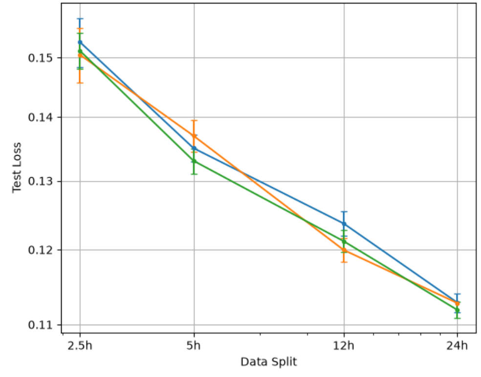
4. Show error bars on the points for your method, where the width of the error bar denotes (two-sided) 95% confidence intervals for the difference to the baseline using your estimates of the effective sample size-corrected standard error.

Example Plot

This is an example of a scaling plot comparing three methods which are not significantly different from each other.

Analysis Questions

First answer the following conceptual questions:

1. Why can't we compute error bars directly using the standard error, std(X) / sqrt(n)? What will happen if we try to do this?

2. Why do we need to do a paired comparison? What would happen if we instead computed the error bars for each method independently, and then compared the two?

   Note

   If you're not sure how to answer these questions from statistical principles, try redrawing your plot according to these alternate methods, and see what happens!

Then, answer the following questions about your proposed change:

1. Is your change significantly better? Is your change better, worse, or statistically indistinguishable from the baseline across the different training set sizes?

2. Does your change scale? Does the gap between the two curves hold, widen, or shrink as the training set grows?

3. As a whole, do you believe your change is an improvement? If so, why? If not, why not?

Finally, reflect on the procedure as a whole:

1. Do you think the evaluation set is the right size? Using your results and/or training curves, argue for whether the evaluation set is too small, too large, or about right.

2. Do you think the validation set is the right size? Using your results and/or training curves, argue for whether 20% is too small, too large, or about right.

Grading and Submission

Submission Checklist

Your submission should include the following:

• Your checkpoint submission (in the separate Canvas assignment): the projects output (or nvidia-smi, if you are using your own compute), and your hello_world.sh job log
• Your lab report, including a description of your proposed change, justification for why this could improve the model's performance, a high level description of your implementation, the scaling plot, and your answers to the analysis questions
• A .tar or .zip archive of your entire repository, including the .git directory, but omitting results/, data/, .venv/, and any other untracked artifacts

Rubric

Warning

Submission of the lab report and code are prerequisites to receiving credit for any component of this lab!

This lab is worth 100 points, divided across five components:

Component	Points
Hello World, HPC!	5
Baseline replication	20
Proposed change	30
Scaling law ablation	20
Analysis and discussion	25

1. Hello World, HPC! (5 points)

   1. (2 points) projects output on Bridges-2, or nvidia-smi on your own compute
   2. (3 points) A hello_world.sh job runs, with its log included; or, if you are using your own compute, the I/Q-1M dataset is downloaded

2. Baseline replication (20 points)

   1. (20 points) Four baseline runs (+split=p10, p20, p50, p100) are reported in your scaling law ablation table and plot (4)

3. Proposed change (30 points)

   1. (10 points) The change is clearly specified, and a reasonable argument is made for why it could improve the model's performance
   2. (10 points) The implementation and configuration files for the change
   3. (5 points) Unit tests are provided
   4. (5 points) Automated quality checks (formatting, type checking, and CI)

   Partial Credit

   Credit for (b), (c), and (d) can only be given if the proposed change involves some substantive code addition or modification (i.e., involves more than a hyperparameter change).

4. Scaling law ablation (20 points)

   1. (10 points) Four experiment runs
   2. (5 points) Error bars are computed as a paired comparison, independently for each split
   3. (5 points) The scaling plot is presented, and meets the stated requirements

5. Analysis and discussion (25 points)

   1. (10 points) Conceptual questions
   2. (10 points) Analysis of the proposed change
   3. (5 points) Data size discussion