Analysis

This page collects the measurements behind the design of iqz, on the two datasets it was designed for: Tartan* and I/Q-1M. Every number, table, and figure here is generated by the analysis/ project in this repository.

Reproducing

The analysis/ directory is a standalone project, with its own dependencies; it reads both datasets only through their official loaders (tartanstar and roverd), so local copies in other supported formats work as well.

cd analysis
uv sync
uv run iqz-analysis all --tartanstar /path/to/tartanstar --iq1m /path/to/iq1m --workers 64

Each step can also be run on its own (uv run iqz-analysis --help); stats and render only need the committed results in analysis/results/.

Results

Datasets

Both datasets record a TI mmWave radar with 3 TX and 4 RX antennas, and store raw ADC samples as little-endian i16 in TI's IIQQ interleave (Q0 Q1 I0 I1 Q2 Q3 ...), with no processing applied.

• Tartan* records continuous chirps: one 3-TX chirp loop per frame, (1, 3, 4, 1024), at 1600 Hz (about 39 MB/s). iqz chunks are 64 consecutive frames.
• I/Q-1M records 64-chirp frames, (64, 3, 4, 512), at 20 Hz (about 16 MB/s); each frame is one chunk. Indoor and outdoor traces use slower chirps than the bike traces.

	Tartan*	I/Q-1M
Traces	340	160
Chunks of 64 chirps	6.97 M	2.09 M
Radar data	10.96 TB	1.64 TB
zstd-3 on raw bytes	1.617× [1.606, 1.627]	1.429× [1.407, 1.448]
iqz	2.312× [2.270, 2.348]	1.839× [1.780, 1.887]
Storage with iqz	4.74 TB	0.89 TB

Ratio

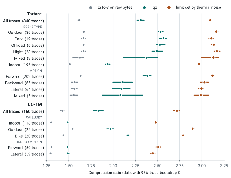
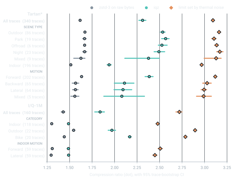
iqz compresses Tartan* by 2.31× and I/Q-1M by 1.84×, against 1.62× and 1.43× for zstd on the raw bytes; thermal noise caps any lossless coder at about 3.1× and 2.7× respectively. Scene type matters most: outdoor-type scenes reach about 2.5× on Tartan* and 2.0–2.2× on I/Q-1M, while indoor scenes compress least on both datasets.

Bootstrapped Confidence Intervals

Ratios are measured on 10,000 chunks of 64 chirps per dataset, drawn uniformly at random from all of the radar data, so traces are represented in proportion to their length.

Chunks from the same trace are correlated, so the intervals are 95% trace-level bootstrap intervals (whole traces resampled 5,000 times); they estimate what to expect on new traces. The table also lists the tighter chunk-level intervals, which describe the datasets as they stand.

Compression ratio by group

Group	Traces	Chunks	zstd-3	iqz	95% CI (traces)	95% CI (chunks)
Tartan*
All traces	340	10,000	1.617×	2.312×	[2.270, 2.348]	[2.304, 2.319]
Scene type
Outdoor	86	4,064	1.671×	2.535×	[2.509, 2.562]	[2.526, 2.544]
Park	19	955	1.666×	2.568×	[2.523, 2.606]	[2.557, 2.579]
Offroad	6	307	1.667×	2.526×	[2.486, 2.584]	[2.511, 2.542]
Night	23	1,156	1.667×	2.493×	[2.440, 2.557]	[2.477, 2.509]
Mixed	9	415	1.626×	2.378×	[2.114, 2.498]	[2.341, 2.415]
Indoor	196	3,038	1.514×	1.940×	[1.917, 1.964]	[1.931, 1.948]
Motion
Forward	202	7,553	1.634×	2.385×	[2.339, 2.428]	[2.377, 2.394]
Backward	65	1,251	1.567×	2.110×	[1.997, 2.215]	[2.090, 2.131]
Lateral	64	1,105	1.565×	2.094×	[1.994, 2.191]	[2.075, 2.113]
Mixed	5	54	1.558×	2.081×	[1.881, 2.332]	[2.013, 2.155]
I/Q-1M
All traces	160	10,000	1.429×	1.839×	[1.780, 1.887]	[1.832, 1.846]
Category
Indoor	118	3,100	1.302×	1.488×	[1.478, 1.498]	[1.484, 1.492]
Outdoor	22	3,713	1.545×	1.970×	[1.929, 2.011]	[1.962, 1.979]
Bike	20	3,187	1.441×	2.168×	[2.152, 2.186]	[2.159, 2.178]
Indoor motion
Forward	59	1,648	1.307×	1.487×	[1.472, 1.502]	[1.482, 1.493]
Lateral	59	1,452	1.295×	1.489×	[1.476, 1.502]	[1.484, 1.495]

Scene type matters most. Outdoor-type scenes compress best, and indoor scenes least on both datasets: indoor clutter is close to the radar, and changes quickly as the rig moves. Groups with fewer than 3 traces count toward "All traces", but have no row of their own; groups with few traces have wide intervals.

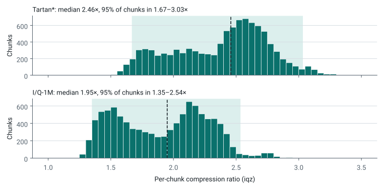
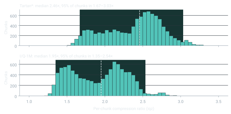
Both per-chunk distributions have a low shoulder of indoor chunks: about 90% of the chunks below 2.0× on Tartan*, and below 1.6× on I/Q-1M, are indoor.

How far can lossless compression go? Thermal noise from the receiver cannot be predicted, so no lossless coder can store it in fewer than log2(σ) + 2.05 bits per value (the entropy of Gaussian noise with standard deviation σ), which caps the compression ratio at 16 / bits. The noise level of every sampled chunk is estimated from its range-Doppler map, which does not require a static scene. The limits are shown in the compression ratio chart above.

Noise limit by group

Group	Noise σ, LSB	Ratio limit	iqz	Gap, bits/value
Tartan*
All traces	8.5	3.094× [3.08, 3.11]	2.312×	1.8
Outdoor	8.0	3.161× [3.14, 3.18]	2.535×	1.3
Park	8.5	3.106× [3.08, 3.13]	2.568×	1.1
Offroad	8.3	3.135× [3.11, 3.15]	2.526×	1.2
Night	8.0	3.169× [3.14, 3.21]	2.493×	1.4
Mixed	8.0	3.129× [3.00, 3.18]	2.378×	1.6
Indoor	10.0	2.968× [2.95, 2.98]	1.940×	2.9
I/Q-1M
All traces	12.9	2.720× [2.68, 2.75]	1.839×	2.8
Indoor	20.6	2.480× [2.46, 2.50]	1.488×	4.3
Outdoor	10.7	2.895× [2.88, 2.91]	1.970×	2.6
Bike	12.9	2.787× [2.78, 2.80]	2.168×	1.6

How is the noise floor estimated?

• Range-Doppler maps. Thermal noise is white, so after a Doppler FFT it spreads evenly over all Doppler bins; scene content does not. Static clutter falls into Doppler bin 0 (which the mean chirp removes anyway), and targets and moving clutter fill only part of the Doppler axis. The noise power of each range bin is estimated from the 10th percentile of its Doppler cells, using the fact that the power of complex Gaussian noise is exponentially distributed.
• Per channel and range. Noise levels differ between the 12 virtual channels (by a factor of about 1.4 typically, and up to 2.5), and across range, where the receive chain's high-pass and anti-alias filters shape the noise. Levels are therefore estimated per channel and range bin; for such coloured noise, the entropy is set by the geometric mean of the levels.
• Contamination. Scene content that fills much of the Doppler axis inflates the estimate, and so lowers the limit. Comparing with the estimate from the median instead of the 10th percentile shows this is small (at most about 5% on any group) except in dense indoor I/Q-1M scenes (about 14%), whose limit is correspondingly conservative.
• Check. iqz never beats the limit: on every one of the 20,000 sampled chunks, it uses at least 0.12 bits per value more than the estimated noise alone.

Speed

Single-threaded throughput, in MB/s of raw data, with data in memory, measured on 200 chunks from the sample.

Implementation	Tartan* encode	decode	I/Q-1M encode	decode
iqz, native (Rust) backend	1,286	3,416	864	2,866
iqz, numpy backend	1,042	2,374	679	2,115
zstd level 3 on the raw bytes, for reference	250	1,355	393	1,817

MB/s of raw data, single thread, data in memory, decoding into a reused output buffer. CPU: AMD EPYC 9575F 64-Core Processor; libzstd 1.5.7.

Ablations & Baselines

All alternatives are measured on the same 10,000 chunks per dataset as the results above, and compared with iqz by their total size ("vs. iqz", with a 95% trace-bootstrap interval; positive is smaller than iqz).

Predictor

Variant	Tartan* ratio	vs. iqz	I/Q-1M ratio	vs. iqz
None (zigzag + shuffle only)	1.993×	−13.8% [−14.5, −12.9]	1.698×	−7.7% [−9.3, −5.9]
Previous chirp (delta)	2.172×	−6.0% [−6.4, −5.6]	1.739×	−5.4% [−6.0, −4.7]
Chunk mean chirp (iqz)	2.312×	—	1.839×	—
Better of delta and mean, per chunk	2.333×	+0.9% [+0.8, +1.1]	1.855×	+0.9% [+0.7, +1.0]
Mean, then delta along fast time	2.225×	−3.8% [−4.1, −3.4]	1.751×	−4.8% [−5.0, −4.5]
Mean, then 2nd-order fixed predictor (fast time)	2.040×	−11.7% [−12.2, −11.3]	1.626×	−11.6% [−12.2, −10.8]
Mean, then 3rd-order fixed predictor (fast time)	1.843×	−20.2% [−20.8, −19.7]	1.509×	−17.9% [−18.8, −16.9]
Mean, then 4th-order LPC per series (fast time)	2.452×	+6.1% [+5.7, +6.4]	1.961×	+6.6% [+6.2, +7.0]
Mean, then neighbouring RX antenna	2.281×	−1.3% [−1.6, −1.0]	1.790×	−2.7% [−2.9, −2.4]
Mean, then neighbouring TX antenna	2.229×	−3.6% [−3.7, −3.5]	1.754×	−4.6% [−4.8, −4.4]

• Previous chirp (delta) puts two chirps' noise into each residual, doubling its variance; the mean chirp adds only 1/64. The delta wins mainly under lateral motion, where static objects acquire a Doppler shift and partly cancel out of the mean.
• Neighbouring antennas: after subtracting the mean, the residual is mostly thermal noise, which is independent across antennas, so differencing them only adds noise.
• Fixed polynomial predictors along fast time amplify the (white) noise.
• Least-squares LPC along fast time (4th order, fit per antenna and I/Q component) is the one predictor that improves on the mean alone, by about 6% on both datasets, and on nearly every chunk. It exploits the colouring of the noise by the receive filters (see Ratio). It requires de-interleaving I and Q, storing coefficients, and adds a serial dependency along fast time to decoding.

Chunk size

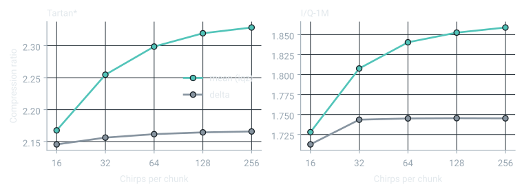
Paired comparison on 1,000 windows of 256 consecutive chirps per dataset: each window is split into chunks of each size, so every size compresses exactly the same chirps. Changes are relative to 64 chirps per chunk.

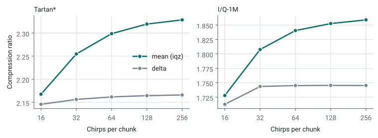
Chirps per chunk	Tartan*, mean (iqz)	Tartan*, delta	I/Q-1M, mean (iqz)	I/Q-1M, delta
16	−5.7% [−5.8, −5.6]	−0.7% [−0.8, −0.7]	−6.1% [−6.2, −6.0]	−1.9% [−1.9, −1.8]
32	−1.9% [−1.9, −1.9]	−0.2% [−0.3, −0.2]	−1.8% [−1.8, −1.8]	−0.1% [−0.1, −0.1]
64	2.299×	2.162×	1.840×	1.745×
128	+0.9% [+0.9, +0.9]	+0.1% [+0.1, +0.1]	+0.7% [+0.5, +0.8]	+0.0% [+0.0, +0.0]
256	+1.3% [+1.2, +1.4]	+0.2% [+0.2, +0.2]	+1.0% [+0.8, +1.2]	+0.0% [−0.0, +0.0]

Larger chunks estimate the mean from more chirps, and amortize its cost over more of them, but with diminishing returns; they also make random access coarser.

Layout

Variant	Tartan* ratio	vs. iqz	I/Q-1M ratio	vs. iqz
Stored order, IIQQ interleaved (iqz)	2.312×	—	1.839×	—
Axis order slow-tx-rx-iq-fast	2.309×	−0.1% [−0.1, −0.1]	1.839×	+0.0% [+0.0, +0.1]
Axis order slow-tx-rx-fast-iq	2.313×	+0.1% [+0.1, +0.1]	1.843×	+0.2% [+0.2, +0.3]
Axis order slow-fast-tx-rx-iq	2.306×	−0.2% [−0.3, −0.2]	1.829×	−0.5% [−0.6, −0.4]
Axis order fast-slow-tx-rx-iq	2.322×	+0.5% [+0.4, +0.5]	1.834×	−0.3% [−0.4, −0.2]
Axis order tx-rx-iq-slow-fast	2.314×	+0.1% [+0.1, +0.1]	1.839×	+0.0% [+0.0, +0.1]
Axis order tx-rx-iq-fast-slow	2.319×	+0.3% [+0.3, +0.4]	1.848×	+0.5% [+0.4, +0.6]
Axis order iq-tx-rx-slow-fast	2.312×	+0.0% [+0.0, +0.1]	1.839×	+0.0% [−0.0, +0.0]
Separate zstd frame per antenna	2.314×	+0.1% [+0.0, +0.1]	1.802×	−2.0% [−2.4, −1.7]
Separate zstd frame per I/Q component	2.308×	−0.1% [−0.2, −0.1]	1.838×	−0.0% [−0.1, −0.0]

zstd effectively codes each symbol on its own, so the order of the axes barely matters (within ±0.5%), and the antennas' statistics differ too little to pay for separate entropy tables. iqz keeps the stored order, which needs no reordering at all.

Entropy coder

Each coder replaces zstd on the same mean residual (zigzagged and byte-shuffled for the byte-oriented coders; as i16 series per antenna and I/Q component for pcodec and FLAC; as 64-chirp tiles per antenna and I/Q component for the image codecs). Decode speeds are for the entropy stage alone (single-threaded), so the coders can be compared with each other; the full decode throughput of iqz, including the inverse transform, is in Speed.

Coder	Tartan* ratio	vs. iqz	entropy decode MB/s	I/Q-1M ratio	vs. iqz	entropy decode MB/s
zstd level 3, on the raw bytes (no transform)	1.617×	−30.0%	1,355	1.429×	−22.3%	1,817
zstd level 3 (as used by iqz)	2.312×	—	3,892	1.839×	—	3,255
zstd level -1	1.914×	−17.2%	10,228	1.670×	−9.2%	5,211
lz4	1.871×	−19.1%	12,596	1.582×	−14.0%	7,669
lzma	2.337×	+1.1%	125	1.881×	+2.3%	154
pcodec	2.366×	+2.4%	2,073	1.899×	+3.3%	2,128
FLAC, level 8	2.498×	+8.1%	309	2.062×	+12.1%	302
JPEG-LS	2.190×	−5.3%	132	1.767×	−3.9%	118
JPEG 2000	2.204×	−4.6%	23	1.782×	−3.1%	20
JPEG-XL	2.287×	−1.1%	40	1.810×	−1.6%	35
HTJ2K	2.094×	−9.4%	798	1.703×	−7.4%	727
Rice coding, best parameter per 512 values (estimate)	2.331×	+0.8%	—	1.867×	+1.5%	—
Bit-packing, width per 128 values (estimate)	2.097×	−9.3%	—	1.727×	−6.1%	—
Order-0 entropy: best symbol-by-symbol coder (bound)	2.358×	+2.0%	—	1.894×	+3.0%	—

zstd at level 3 lands within 2–3% of the best any symbol-by-symbol coder could do on these residuals (the order-0 entropy bound); lzma and pcodec gain a similar amount, at a fraction of the decode speed. FLAC, which adds its own adaptive linear prediction, compresses 8–12% further, much like the LPC predictor above, but decodes more than 10× more slowly.

zstd level

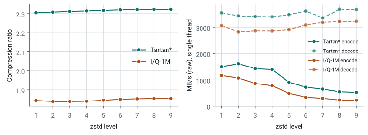
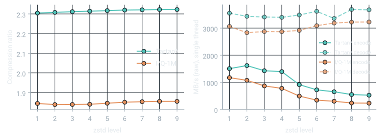
Compression ratio and speed by zstd level

zstd level	Tartan* ratio	encode MB/s	decode MB/s	I/Q-1M ratio	encode MB/s	decode MB/s
1	2.304×	1,503	3,551	1.844×	1,169	3,061
2	2.308×	1,616	3,434	1.839×	1,071	2,831
3	2.312×	1,425	3,409	1.839×	864	2,872
4	2.314×	1,392	3,397	1.840×	774	2,868
5	2.317×	912	3,484	1.845×	489	2,914
6	2.320×	719	3,619	1.851×	339	3,088
7	2.321×	648	3,355	1.853×	298	3,186
8	2.322×	545	3,687	1.855×	233	3,221
9	2.322×	522	3,675	1.855×	228	3,226

The level barely affects the ratio or the decode speed, while encoding slows down substantially at higher levels.